Many students of calculus learn of Newton's method for approximating solutions of equations of the form
f(x)=0
where f is a continuous, once differentiable function of the real numbers. To review: the idea is that one has a real number a and wants to find a point a' which is closer to a solution. If f were linear, then it would be trivial: just take the tangent to the graph of f at (a,f(a)) and see where it intersects the x-axis. The tangent has the equation
y - f(a) = f'(a)(x - a).
To find the intersection of this line with the x-axis, set y to 0 in the equation above and solve for x:
x = a - f(a) / f'(a).
Note that this requires that f'(a)≠0. If this is not the case, then the tangent is horizontal and one cannot make any progress towards finding a root. One must simply find a new starting-point and start over.
When f is not linear, this unfortunately does not in general give a solution. However, if a is already not too far from a solution, then the solution x of the above equation should be at least closer to an actual solution.
With this ansatz we construct an iterative process as follows. We pick some starting-point a0 and, for each iterate an, n≥0, we compute an+1 iteratively via
an+1 = an - f(an) / f'(an).
We stop when f(an) is sufficiently small or (with failure) if f'(an) is zero.
This begs a question: in general there are possibly many solutions to the equation f(x)=0. The behaviour of the iteration is determined completely by the choice of starting-point a0. So to which solution does the iteration converge for a given choice of starting-point? Does it converge to a root for all choices of starting-point, and if not, for what points does it not converge?
The latter part of the question we can already answer in the negative: as already mentioned, when f'(an) is zero, we can make no further progress. Furthermore, perhaps f(x)=0 has no real solutions at all! For example, for no starting-point a_0 can the iteration with f(x)=x2+1 converge to a root, that function having no real roots. The masochistic among you might wish to see what happens when you run this iteration for such a function. To be safe from such pathologies, we terminate the iteration with failure when n is sufficiently large, say, over 1000, without having shown a sign of convergence.
The former question is quite interesting and ties into some fascinating branches of higher mathematics, including topology and fractal geometry. In this post I will describe how to write a script in Python to visualise its answer.
First, observe that the entire method described above works just as well if we work over the complex numbers and allow a0 to be and point in the complex plane C. Here we must restrict our attention to functions which are holomorphic in at least some subset D of C, which we will take to be a rectangle which can be nicely displayed on the computer-screen. Polynomials in one variable are perfect for this, though other functions can be used as well. For simplicity, however, we'll restrict our attention to polynomials.
The idea of the Python-script is as follows: we define a polynomial function of one (complex) variable and a rectangle in the complex plane, along with a vertical and horizontal resolution. We also create a canvas with size equal to the aforementioned resolution. This defines a grid in that rectangle and, for every vertex on the grid, we run the Newton-iteration with that vertex as a starting-point and see whether and to which root the iteration converges. If the iteration converges to a root, we paint the point with a colour which corresponds to that root. If the iteration does not converge at all, we paint the corresponding point on the canvas black.
Let's get started. We need first a few tools for working with polynomials. We'll represent a polynomial just as a list of its coefficients, that is, the polynomial
f(z)=a0+a1x+a2x2+...+anxn
will be represented via a Python-list as
[a_0,a_1,...,a_n]
We need a function to evaluate such a polynomial at a point. We just use Horner's method.
def eval (poly, x):
    res = 0
    for a in reversed (poly):
        res = res * x + a

    return res
Now we need to be able to construct the derivative of a polynomial. One learns this in precalculus.
def differentiate (poly):
    dpoly = [n * a for n, a in enumerate (poly)]
    dpoly.pop (0)   # Shift degrees down by one
    return dpoly
Now we define an exception which is thrown when the process fails due to a bad choice of starting-point.
class bad_start_point (Exception):
    pass
Now we are ready for the Newton-iteration itself.
def newton (f, a_0, tolerance = 1e-5, max_iter = 100):
    a_n = a_0
    df = differentiate (f)

    try:
        for n in range (max_iter):
            if abs (eval (f, a_n)) < tolerance:
                # Root found. Return.
                return a_n

            a_n = a_n - eval (f, a_n) / eval (df, a_n)

    except ZeroDivisionError:
        # Tangent was zero
        pass

    # If we reach this point, the iteration has failed
    raise bad_start_point
Once we have run the Newton-iteration on a point, and supposing that the iteration actually converges, we need a way to identify which colour to paint the root. Since we don't know the roots in advance, we'll take a rather lazy approach: we take a list of colours, paint the first root which we find with the first colour on the list, the second with the second, and so on.
Let's first define a class which defines a colour via red, green, and blue components.
class colour:
    def __init__ (self, red, green, blue):
        self.red = red
        self.green = green
        self.blue = blue
Now we make a list of colours.
colour_list = [
    colour (1.0, 0, 0),
    colour (0, 1.0, 0),
    colour (0, 0, 1.0),
    colour (1.0, 1.0, 0),
    colour (1.0, 0, 1.0),
    colour (0, 1.0, 1.0),
    colour (0.5, 0.5, 0.5)
]
Finally we need a function which identifies the colour of a point by root, adding new roots as needed.
def identify_root (roots, r, tolerance = 1e-4):
    for root, colour in roots.iteritems ():
        if abs (root - r) < tolerance:
            return colour

        # root not found among existing roots
        roots[r] = colour_list.pop (0)
        return roots[r]
If two roots are within the parameter tolerance of one another, then they are deemed to be the same. The correct choice of tolerance is actually quite tricky, so we just go with a simple rule which will work in most cases. The parameter roots is a hash which assigns a colour to each root.
Armed with this, we can write a program which runs the Newton-iteration on each point of the grid.
def newton_grid (f, xmin, ymin, xmax, ymax, xres, yres):
    # Construct xres x yres array
    grid = [[0 for y in range (yres)] for x in range (xres)]
    roots = {}

    for x_idx in range (xres):
        for y_idx in range (yres):
            x = xmin + (xmax - xmin) * x_idx / xres
            y = ymin + (ymax - ymin) * y_idx / yres
            a_0 = complex (x, y)

            try:
                r = newton (f, a_0)
                grid[x_idx][y_idx] = identify_root (roots, r)

            except bad_start_point:
                grid[x_idx][y_idx] = colour (0, 0, 0)

    return grid
The function returns a two-dimensional array of colour-objects.
Now we have the grid with its colours and would like to paint it onto something. We use the library Cairo for this (see here for the Python-bindings).
import cairo

def draw (cr, grid):
    for x_idx, y_list in enumerate (grid):
        for y_idx, colour in enumerate (y_list):
            cr.set_source_rgb (colour.red, colour.green, colour.blue)
            cr.rectangle (x_idx, y_idx, 1, 1)
            cr.fill ()
The parameter cr is a Cairo context-object which we construct next. The parameter grid is our aforementioned grid.
Finally we write the main routine which creates the Cairo context-object, computes the colours, draws the canvas, and writes everything to an output-file. In this example we use the polynomial x3-1 and consider the rectangle from (-2,-2) to (2,2). One can easily change these things.
def main (argv):
    xres = 500
    yres = 500

    f = [-1, 0, 0, 1]  # x^3 - 1
    grid = newton_grid (f, -2.0, -2.0, 2.0, 2.0, xres, yres)
    surface = cairo.ImageSurface (cairo.FORMAT_ARGB32, xres, yres)
    cr = cairo.Context (surface)
    draw (cr, grid)
    surface.write_to_png ('output.png')
    return 0
The chosen polynomial has three roots which are arranged in an equilateral triangle centred on the origin with vertices on the unit circle and pointing to the right.
When one runs this with the above parameters, the output is surprisingly complex.
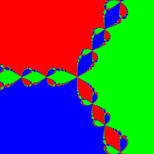
As one would expect, close to the roots themselves, everything converges quickly. The boundary-zones between these basins are where things become interesting. The border shows a lot of complexity and self-similarity which is common to fractal-geometry.
One other thing one notices: not much black. So this phenomenon that the starting-point is "bad" doesn't seem to occur so often. Is this generally true? Let's try with the polynomial x4-4x2+5x+2.
Seems to suggest that not converging is actually quite unusual (as long as there are roots to which to converge!). So I end this post with a question:
Question: For what functions f(x) does the set of starting-points a0 for which the Newton-iteration fails to converge have measure 0?
Appendix: Here is the Python-script in its entirety
import sys
import cairo

class colour:
    def __init__ (self, red, green, blue):
        self.red = red
        self.green = green
        self.blue = blue

# Global list of colours
colour_list = [
    colour (1.0, 0, 0),
    colour (0, 1.0, 0),
    colour (0, 0, 1.0),
    colour (1.0, 1.0, 0),
    colour (1.0, 0, 1.0),
    colour (0, 1.0, 1.0),
    colour (0.5, 0.5, 0.5)
]

class bad_start_point (Exception):
    pass

def eval (poly, x):
    res = 0
    for a in reversed (poly):
        res = res * x + a

    return res

def differentiate (poly):
    dpoly = [n * a for n, a in enumerate (poly)]
    dpoly.pop (0)
    return dpoly

def newton (f, a_0, tolerance = 1e-5, max_iter = 100):
    a_n = a_0
    df = differentiate (f)

    try:
        for n in range (max_iter):
            if abs (eval (f, a_n)) < tolerance:
                # Root found. Return.
                return a_n

            a_n = a_n - eval (f, a_n) / eval (df, a_n)

    except ZeroDivisionError:
        # Tangent was zero
        pass

    # If we reach this point, the iteration has failed
    raise bad_start_point

def identify_root (roots, r, tolerance = 1e-5):
    for root, colour in roots.iteritems ():
        if abs (root - r) < tolerance:
            return colour

    # root not found among existing roots
    roots[r] = colour_list.pop (0)
    return roots[r]

def newton_grid (f, xmin, ymin, xmax, ymax, xres, yres):
    # Construct xres x yres array
    grid = [[0 for y in range (yres)] for x in range (xres)]
    roots = {}

    for x_idx in range (xres):
        for y_idx in range (yres):
            x = xmin + (xmax - xmin) * x_idx / xres
            y = ymin + (ymax - ymin) * y_idx / yres
            a_0 = complex (x, y)

            try:
                r = newton (f, a_0)
                grid[x_idx][y_idx] = identify_root (roots, r)

            except bad_start_point:
                grid[x_idx][y_idx] = colour (0, 0, 0)

    return grid

def draw (cr, grid):
    for x_idx, y_list in enumerate (grid):
        for y_idx, colour in enumerate (y_list):
            cr.set_source_rgb (colour.red, colour.green, colour.blue)
            cr.rectangle (x_idx, y_idx, 1, 1)
            cr.fill ()

def main (argv):
    xres = 500
    yres = 500

    f = [2, 5, -4, 0, 1]  # x^4 - 4x^2 + 5 x + 2
    grid = newton_grid (f, -2.0, -2.0, 2.0, 2.0, xres, yres)
    surface = cairo.ImageSurface (cairo.FORMAT_ARGB32, xres, yres)
    cr = cairo.Context (surface)
    draw (cr, grid)
    surface.write_to_png ('output.png')
    return 0

if __name__ == '__main__':
    sys.exit (main (sys.argv))