This is part one of a three-part series on my experiments working with machine learning in Rust and its ecosystem. This installment discusses my motivation this topic as well as its theoretical underpinnings. In the second installment, I will discuss what crates exist to do machine learning in Rust. The third installment will discuss the results of my experimentation in the area.
Backstory
One day a few months ago, I was feeling the itch to build something interesting in Rust in my spare time. I decided to try to implement a modern version of a strategy game which I had played in my youth.
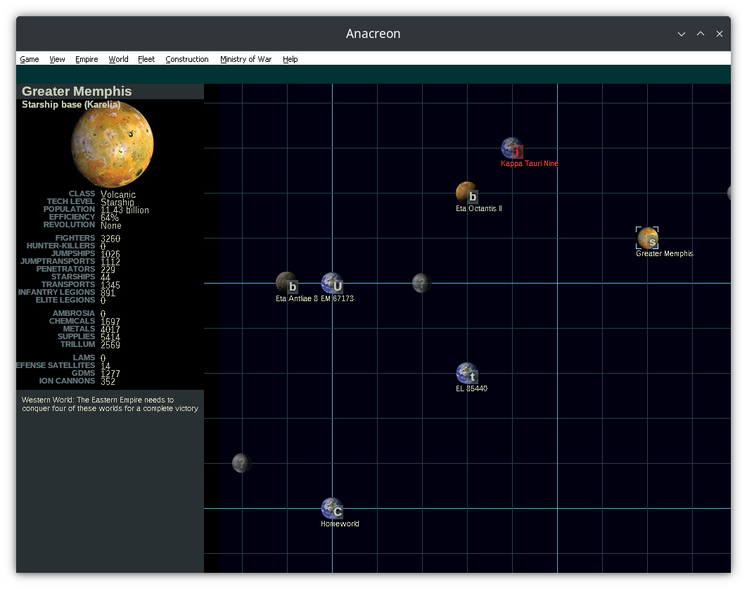
Building such a game is mostly pretty easy. The game mechanics come in lots of little bite-sized chunks. There are no complex graphics or sounds to produce. One can easily add bits and pieces to the game whenever one has an hour of free time. It’s not too mentally taxing. This makes it a great hobby project.
But there’s one component which isn’t so straightforward, one which requires real design and careful thinking: the computer player AI.
Back in the 1980s and 1990s when my game’s antecedent was developed, it was common to use expert systems. This just means that the code controlling the computer player consists of fixed rules and heuristics which the game developer thought out. The algorithm is fixed ahead of time.
Writing expert systems well is a really tedious undertaking. It’s hard to tune them so that the computer behaves in a “believable” way and really challenges the player. Even if one succeeds, the player eventually understands enough about how the AI player works to outsmart it. The game becomes boring with time.
How do we solve such problems now, in the 2020s? Machine learning, of course!
When you don’t know how to solve your problem, that’s when you use machine learning.
– a former Google colleague of mine
A short primer on machine learning
I start with a general introduction to machine learning and specifically deep learning. Those who are familiar with the subject can skip to the following section. For those who would like to learn more, I recommend the following resources:
- the Coursera specialization from Stanford University,
- Serrano Academy from a former university colleague of mine.
Machine learning is really just data-driven programming, as I explain below.
We want to estimate some function \(f\). For example, \(f\) might map the pixels of an image to a natural langauge description of that image. Or, as in the case of generative AI systems such as Stable Diffusion, it might be the inverse of that.
We start by defining a model \(\hat{f}\) which estimates \(f\). Its definition includes a whole bunch of tunable numbers called parameters. We train \(\hat{f}\) by adjusting the parameters to improve the estimate of \(f\).
We define a cost function \(C\). Given a model \(\hat{f}\) and some set of inputs \(I\), \(C(f, \hat{f}, I)\) is a number showing how much the inferred \(\hat{f}(I)\) and the true \(f(I)\) differ. A common choice of cost function is mean squared error:
\[C(f, \hat{f}, I) = \frac{1}{|I|}\sum_{v\in I}(f(v)-\hat{f}(v))^2\]
Different values of parameters produce different costs for a given set of input data, so one can graph the cost function against the parameter values:
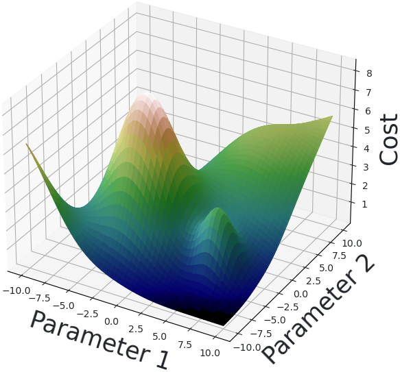
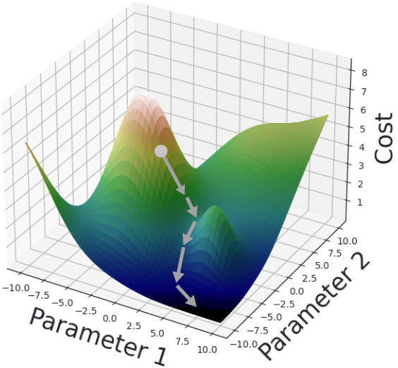
We train \(\hat{f}\) by an iterative process called gradient descent. In each iteration, we select various inputs \(I\), called training data, for which we know the true values \(f(I)\). Using this knowledge, we calculate the cost \(C(f, \hat{f}, I)\) as well as the direction in which we must move the parmaeters to reduce the cost the most. We move the parameters a bit in this direction, then repeat. The cost should fall on each iteration until it approaches a minimum.
The use of training examples is where the data-driven aspect comes in: we train the model by collecting reams of real-world example data which we use to refine our model.
We may evaluate \(\hat{f}\) to see how well it estimates \(f\) in its current parameter state. To do this, we pick a different set of inputs \(J\), called test data, for which we also know the true \(f(J)\). We compute the cost \(C(f, \hat{f}, J)\) of these test data. A cost which is much greater than that of training data indicates overfitting: the model trained too much on specific data and cannot generalize to different inputs. If the cost of both the test and training data are too high, then we have underfitting. These problems can be addressed with various techniques, such as adjusting the model and obtaining more training data.
When the model performs adequately during evaluation, we begin to apply it to real world data. This is called inference.
Neural networks
How to we define our model? Nowadays a great deal of machine learning is done with neural networks. While that sounds quite fancy, the concept is remarkably simple. They have become so popular because of their flexilibity: they can model almost any function with arbitrarily high precision.
The function \(f\) maps an array of floating point numbers to another array of floating point numbers. The model maps the input through a series of layers: simple functions typically defined via trainable parameters. The inputs and outputs of these layers are sometimes called neurons. A typical layer is the composition of two functions:
- multiplication by a matrix whose entries are trainable parameters, and
- a nonlinear activation function.
All layers except the last, which generates the model output, are called hidden layers.
A dense layer makes all entries in the matrix trainable. Some architectures, such as convolutional neural networks, restrict the matrices in some layers so that most entries are zero. This technique is widely used in image recognition applications, for example.
A popular choice of activation function is the rectified linear unit or ReLU:
\[\text{ReLU}(x)=\begin{cases}0,& \text{if}\ x < 0,\\x,&\text{otherwise.}\end{cases}\]
The activation function is what makes the entire neural network nonlinear. If it weren’t present, then the whole network would just collapse into a single matrix multiplication. It would only be able to approximate functions which are almost linear themselves. Adding a nonlinear activation function allows a suitable neural network to approximate an arbitrary function to arbitrary precision.
In fact, it suffices to have a single hidden layer to model any function to arbitrary precision! But one would need a lot of neurons in general. Adding more intermediate layers can reduce the number of neurons needed exponentially to achieve the same results. However, too many intermediate layers can also make it harder to train the network. Balancing all needs when constructing a neural network is one of the arts of the field.
The choice of which layers exist and how they are set up is called the architecture of the model.
To sum up, we need the following ingredients to use machine learning:
- A function we want to approximate,
- An encoding of both the input and the output of the function as vectors,
- A cost function which measures how good the approximation is,
- A (large) dataset of inputs with their respective true function values.
We then choose the architecture of our model and initialize it. We split the inputs into training and test data and run the training algorithm based on gradient descent.
In the next section, we apply this method to building a computer player AI for a game.
Training a computer to play a game
Machine learning has famously been used to train computer players. Probably the best known example is AlphaGo by Google DeepMind, in which a highly trained neural network beat the the world’s top players at the game of Go. Another example is a model which learnt to play a “jump and run” style video game to the same level as an adolescent human. Its only foreknowledge of the game was the score and the existence of input controls.
We’ll be using a similar – but greatly simplified – approach to that of AlphaGo.
We’ve talked about machine learning in general. To apply what we have discussed to computer players, we need to answer a few questions:
- What function do we model, and how does it relate to gameplay?
- How do we train the model? In particular, how do we get training data?
We’ll start with some terminology. A game has a state which evolves as the players take actions. An action moves the game from one state to another. That change in state may have a stochastic component. A state is terminal when it marks the end of the game.
Some states have an associated reward for a given player. A higher reward implies a more desirable state for the player. A reward can also be negative indicating that the state is undesirable for the player. For example, a winning state for player A has a positive reward for that player but a negative reward for all other players.
The value of a state
The value of a state to a given player is the expected reward the player eventually gets after starting from that state. This depends on a few factors:
- the state itself,
- the strategy the player follows,
- the strategy the player’s opponents follow, and
- any randomness in the game itself.
In determining a state’s value, future rewards may be discounted. Then the same reward implies a higher value if it occurs in the very next state than it would many states later. The degree of discount is a parameter one can set when building the computer player AI. A higher discount implies a more “impatient” player which “wants” to win quickly.
As you might imagine, the value of a given state is practically impossible to compute in general. In terminal states, it’s easy: just take the reward in that state.
In near-terminal states, where the final action is clear, it’s also not too hard. The player will presumably make the best move it can, meaning that it will receive the reward of the resulting terminal state.
The further away one is from a terminal state, the harder it is to calculate the value. In the initial state of a non-trivial game, it’s utterly infeasible to compute directly.
Nevertheless, if we did know how to compute the value of a state, we’d have a nice strategy for the computer AI. For each possible action, compute the value of the state one gets by taking that action. Then take the action which yields the highest value.
The action-value function
With this in mind, we define the function we’re going to model. The action-value function or \(Q\)-function is a function of a state \(s\) and and action \(a\). Taking action will result in a new state \(s'\). Depending on the game, \(s'\) may be randomly determined. Nevertheless, one can talk about its expected value. The \(Q\)-value is thus the expected value of \(s'\).
This answers the first question above: we model the action-value function. Armed with that model, our computer player AI picks the action with the highest estimated \(Q\)-value from the current state. This technique is called Q-learning.
Training the action-value function
Now we move on to the second question above: how do we train our model to approximate \(Q\)?
As discussed above, we need training data to train the model. This means we need states, actions, and their associated \(Q\)-values. But, as we also discussed, it’s practically impossible to know the true value of a state, except in a few trivial cases. So what do we do?
The solution is “fake it until you make it”.
We start with a formula for \(Q\) called the Bellman equation:
\[Q(s, a) = R_{s'} + \gamma \max_{a'} Q(s', a')\]
Here \(R_{s'}\) is the expected reward from the resulting state \(s'\) and \(\gamma\in(0,1]\) is the discount factor. This just says that the \(Q\)-value is what we get if we take the given action and then play optimally according to our strategy from then on.
We’ll use this equation to compute “true” \(Q\)-values for our training examples. We can compute resulting state \(s'\) easily. We can also compute the reward \(R_{s'}\) easily by examining the resulting state. The discount factor \(\gamma\) is fixed.
But what about \(Q(s', a')\)? That’s just another \(Q\)-value, so we seem to be stuck again.
The trick is to estimate \(Q(s',a')\) using our existing model. It’s a terrible estimate at first, but it turns out that (hopefully), the model does eventually converge on the real value of \(Q\).
Bringing it all together
With all that theory, here’s how we proceed to build and train our computer player AI.
First, we define a model. This means defining:
- How the state and actions are encoded as vectors,
- The model architecture, that is, what layers exist and their configurations.
In practice, our model for the action-value function outputs a vector containing the \(Q\)-value of every possible action from that state. That way, the model can be evaluated once and the highest \(Q\)-value just read off the output.
Then we let this model play games. Lots of games. These games produce lots of examples of the form: I started in state \(s\) and took action \(a\). I then found myself in state \(s'\), and (maybe) got reward \(R_{s'}\).
We use these thousands of examples to build training data using the trick with the Bellman equation. These training examples then train the model itself. Rinse, lather, and repeat.
From theory to practice
To build a reinforcement learning system which performs adequately, we need a few more tricks.
Training adversarial games
The method described above works well when the player competes with the “world”. This is the case with many traditional video games, for example.
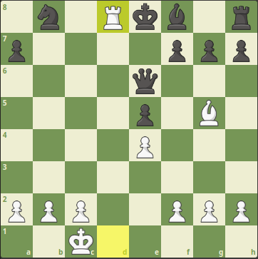
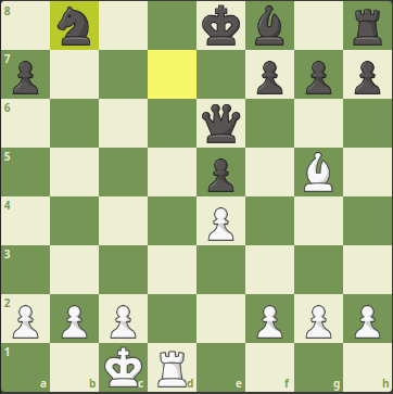
How do we handle adversarial games like Chess? We then need another player against which the player being trained plays. For thousands of games.
One solution is to have the model play against a prior version of itself. It trains for a few hundred games. Then we make a copy of the model and have the opponent use this copy. One variant on this is to evaluate the model against its prior self at the end of each training round, only updating the opponent model if the current one is clearly superior. This is roughly the strategy which DeepMind used to train AlphaGo.
We need to be careful with the encoding of states. One might be tempted to use a state encoding in terms of fixed players such as “white” and “black” in chess. But then the model would always decide in “favour” of the player being trained, even if it is supposed to act on behalf of the opponent player. Thus the state encoding must be expressed in terms of the “current” and “opponent” players.
A challenge with adversarial games is that the definition of the value of a state necessarily depends on the behaviour of the opponent. So training an adversarial game necessarily runs the risk that the model learns to play extremely well against exactly one kind of opponent and no other. We may address this by having the agent train against various opponent models, including a completely naive model which just acts randomly.
Exploration and exploitation
Our technique risks becoming stuck in a local minimum. The model eventually learns to prefer certain moves so much that it can no longer explore the state space.
To overcome this, we let our training agent sometimes deviate from the model. We define a parameter \(\epsilon\) between 0 and 1. For each training game move, with probability \(\epsilon\), the model picks an action at random rather than using the model. The resulting move is probably fantastically stupid. But it helps the model explore more of the state space and therefore learn better. Such a move is called exploratory, while a move determined by the model is called exploitative.
Exponential moving average
Using the method as described thus far, the model will be really unstable. Its behaviour quickly begins to swing wildly from one round to the next. Its performance quickly stops consistently improving and also begins to swing wildly.
This the Achilles heel of our “fake it until you make it” trick using the Bellman equation. The model keeps changing, so the \(Q\)-estimates used to calculate training data keep changing with it. (Perhaps this is an elementary example of model collapse.)
To address this, we introduce exponential moving average. We keep two copies of the model: one to be trained on new training examples, one to be used to compute the \(Q\)-value estimates. Every so often, we update the latter with a weighted average of itself and the former. The weight on the training model may be quite small, say, 0.01. This slows down model convergence considerably, but makes the model more stable. So it’s a tradeoff which is regulated by the weight.
Learning more
I have only scratched the surface of the topic of reinforcement learning here. To learn more, I recommend the book Reinforcement Learning: An Introduction by Richard Sutton and Andrew Barto.
Conclusion
In this article, we looked at how I got started with machine learning in Rust. We then discussed how machine learning works in general and how reinforcement learning can be used to train a model to play games.
In the next installment in this series, I’ll write about the tools of the Rust ecosystem with which we can implement all of this. Stay tuned!